For the course MATH179: Projects in Computational and Applied Mathematics at UCSD, I spent some time looking into accelerating ODE boundary value problem solvers on an FPGA. Unfortunately, this took place before I had learned of HLS, so it was written entirely in Verilog. I have slightly adapted my report for that course below to hopefully show some general practices about how FPGAs can be applied to HPC tasks. It is definitely worth noting that due to time constraints, this problem is very contrived, as linear ODE BVPs can be solved directly. However, the idea of using FPGAs for PDE BVPs with somewhat similar techniques is an active area of research.

Introduction⌗

The example problem in our implementation is the linear boundary value problem.

$$\begin{cases} y’’ - y = 0 \\ y(0)=1 \\ y(8)=0.5 \end{cases}$$

This system can easily be solved analytically, and therefore is a good benchmark to verify the accuracy of our implementation. There are many ways in which to construct an iterative solver for this system. Due to the numerical instability inherent to the system as well as ease of development, we opted for a finite difference method for discretization followed by a basic Jacobi solver.

The FDM is identical to the method presented in these course notes which we will briefly outline. By taking the Taylor expansions of $y(t)$ and rearranging terms to approximate the second derivative we arrive at

$$\frac{y(t + h) - 2y(t) + y(t - h)}{2h} - y(t) = 0$$

When using a discretization such that $x_{i+1} - x_i = h$ this can be written

$$\frac{y_{i+1} - 2y_i + y_{i-1}}{2h} - y_i = 0$$

By combining these approximations to the system at each point in the domain together, we get a banded square matrix with as many columns and rows as there are points in the domain. This matrix also has only one non-zero entry on the diagonal in the first and last rows, to account for the boundary conditions. Constructing a Jacobi iteration scheme based on this matrix leads to the following equations

$$\hat{y_{i}} = \begin{cases} 1 & i = 0 \\ (y_{i-1} + y_{i+1}) \times (2 + h^2)^{-1} & 0 < i < n \\ 0.5 & i = n \end{cases}$$

Where $\hat{y}$ represents the next iteration’s approximation in the algorithm. Note that this computation requires only a single multiplication and addition per index per iteration, which lends well to FPGA implementation.

Data Types and MATLAB Simulation⌗

Unlike traditional processors and GPUs where computations are most efficient when using the native bit-width of the system or floating point, FPGAs have much more flexibility to use smaller data types when this level of precision is not necessary. Using smaller data types leads to less area utilization and power usage. The relative lack of dedicated floating point hardware on FPGAs has also led to a wide adoption of fixed-point arithmetic for applications in DSP, control systems, and others. These fixed-point data types use a set amount of bits in the number for the integer portion, and the rest for the fractional part. For example, a common fixed-point data type used in FIR filters is “Q15”, which uses 16 bits to represent a signed number from -1 to 1 with an epsilon of $2^{-15}$.

For the purposes of this linear solver, we simulated the algorithm in MATLAB using a variety of data types in order to determine the necessary precision for the algorithm to converge. What we found was that a Q4.12 fixed point representation was sufficiently precise for the algorithm to remain stable. The main bottleneck in this regard is the very small intermediary value in the calculation of the second derivative approximation as the number of points in the discretization increases.

Additionally, in MATLAB we tested to see if the SOR algorithm could be utilized to improve on the convergence time of the Jacobi iteration. Unfortunately, the system is only slightly diagonally dominant, and SOR does not converge for any relaxation factor $\omega > 1$ in fixed point arithmetic.

System Architecture⌗

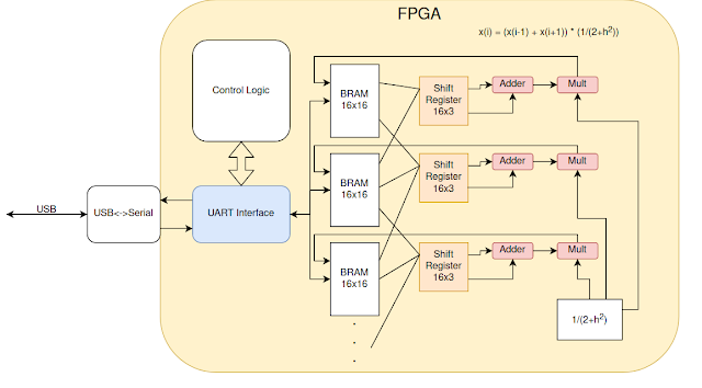
The general architecture for our implementation involves using the existing DSP resources on the FPGA and controlling them using logic in the fabric described with Verilog HDL. The data is sent and received from the interface computer using serial over USB. The current approximation is stored in a series of dual port block RAM resources. The current implementation for the example ODE involves a 128 point uniform discretization, with 16 points stored in each BRAM, and one DSP slice per BRAM. As shown in the above figure, each DSP slice is connected to the BRAM before and after it. This allows for sampling the indices just before and after the first and last index stored in the BRAM, which is necessary for the algorithm. It would be easy to scale this approach to much larger domains, the only limitation being the number of DSP slices, BRAMs, and the capacity of each BRAM.

The goal of using multiple BRAMs is to overcome the main bottleneck on multicore processor setups: the DRAM bus bandwidth. While caching and other techniques have aided this issue in other computational problems, linear solvers generally are still limited by the number of reads per cycle. By using an FPGA we can read and write a very large number of data points per clock cycle, removing this bottleneck.

Through the use of extensive pipelining, the task interval is shortened to only one cycle for computing a single new approximation value. Since all BRAM and DSP pairs can be operated in parallel, this leads to 24 cycles per iteration.

Results⌗

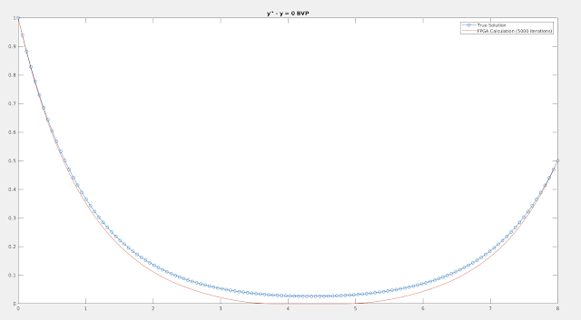
Due to the fixed point arithmetic being used on the FPGA, we did not expect that the results would exactly match the analytical solution. For our purposes, we ran 5000 Jacobi iterations and compared the boundary value problem solution to a result computing in MATLAB.

The computed solution of the FPGA is generally correct, but there is a large amount of error for $y$ close to $0$. We think this is because of the uneven rounding in the multiplication and addition. When multiple adjacent values of $y$ become $0$, this is a steady state for the algorithm since the next approximation is computed as a linear combination of its neighbors. This fact combined with rounding toward 0 in all cases is our hypothesis as to why this phenomenon occurs.

Performance on the FPGA for domains this size is primarily limited by the slow serial communications between computer and FPGA used in our current implementation. However, in more advanced implementations with different hardware busses this is an easy limitation to overcome. Therefore we will focus on the computational speed only in our analysis. The FPGA we are currently testing on (a Xilinx Artix 7 on a Basys 3 development board) has a clock speed of 100MHz. Accounting for 24 clock cycles per iteration with 5000 iterations required, the full computation is completed in 1.2ms. Using the current design, the domain could be increased to 1280 points without any loss in speed by using more area. Further extensions of the domain would scale linearly from this point, until the BRAM capacity on the FPGA is reached.